Spatial Data: The Structure of Geospatial Information
Before we can map our data, we need to understand that geographic information is more than just a table of numbers: it’s a representation of our three-dimensional world projected onto a flat screen. Understanding the principles of how we digitalize physical space is the key to avoiding distorted shapes and misaligned points.
In this lesson, we’ll explore the fundamentals of spatial data structuresusing the sf package. We’ll look at how different geometric shapes are organized, decipher the metadata that gives coordinates their identity, and examine the trade-offs involved in flattening our planet for the digital canvas.
🗺️ Where We Live, But in 2D
In standard data visualization, we map variables to x and y positions on a grid. In spatial visualization, we do the same, but with a crucial difference: our "data points" are not always points, but may represent complex shapes that exist on a curved surface.
To represent our three-dimensional world on a two-dimensional canvas, we most commonly use a vector model . While some spatial data is stored as a grid of pixels (known as raster data), we focus on the vector approach. This model organizes coordinates into specific geometric structures that allow us to map physical boundaries and locations onto a digital 2D grid.
🧱 The Building Blocks
Within the vector model, most spatial datasets you’ll encounter are built from one of three fundamental geometric structures. These are the "Building Blocks" of any digital vector map:
No matter which of these, every shape can essentially be presented by coordinates. Even the most complex border is just a list of numbers organized by these rules:
- Point:
(X, Y)⇒ a single coordinate - Line:
((X1, Y1), (X2, Y2), ...)⇒ a sequence of points - Polygon:
((X1, Y1), ..., (X1, Y1))⇒ a sequence forming a ring
Things often get more complex when we deal with Multipart Geometries as a geographic entity rarely fits into a single simple shape.
🧩 Complex Shapes, Simple Features
A country like Greece or the United States isn't one single polygon. It is a collection of mainlands and various islands that all belong to the same data entry.
In a digital map, we treat these as a single "feature". This ensures that when you look for "Greece" in a dataset, you aren't just getting one island, but the entire country as a unified piece of information.
This is the core of modern spatial data: instead of managing separate lists for your data and your shapes, the standard workflow treats geographic boundaries just like any other variable.
It’s a standard rectangular, two-dimensional table where every row is a geographic feature (like a single location, a river, or a city), and one special column holds the precise instructions on how to draw it.
This approach actually allows you to mix types in a single table. You could have a point (location), a line (river), and a polygon (city) all living in the same dataset, though in practice, we often keep them in separate datasets for clarity to maintain thematic focus and make styling each layer easier.
This "Table with one special column" model isn't just a clever idea: it is a formal international standard called Simple Features .
This standard defines how digital geometries should be stored and described so that different software can "talk" to each other. Whether you are using a GeoJSON file in a web browser, a PostGIS database, or a Shapefile in a GIS, the data follows the same geometric hierarchy.
You might hear spatial data referred to by many names depending on where it is stored, and it can be a bit overwhelming at first. So let's introduce the main file formats briefly:
- GeoJSON: A text-based format popular for web maps and APIs (it looks a lot like a nested R list).
- GeoPackage (.gpkg): The modern, open-source successor to the old "Shapefile" (.shp), much faster and easier to share as a single file.
- Shapefile (.shp): The "grandfather" of spatial formats. While it is still everywhere, it’s actually a collection of at least three different files (
.shp,.shx,.dbf) that must stay together to work. - PostGIS: A powerful spatial extension for SQL databases used by professional cartographers and analysts.
- KML/KMZ: The format used by Google Earth. While great for visualizing points in a browser, it can be a bit "messy" to clean and process for statistical analysis.
And to decode a bit more of the jargon: if someone mentions a "Web Feature Service" (abbreviated as "WFS" or sometimes "WMS"), that person is not actually talking about static files, but a way to provide information. Think of them as a "live stream" of spatial data that you connect to via a URL rather than downloading a file.
The good news? They all "look and feel" the same once you bring them into R.
🪪 Identity Check
Every Simple Features dataset also carries a piece of metadata, essentially a spatial passport, that tells the computer how to interpret the numbers in the table.
A standard spatial header includes:
- Geometry Type: What is the geometric structure, are these points, lines, or polygons?
- Bounding Box: What are the maximum and minimum coordinates of the data?
- CRS: Which spatial representation are these coordinates using? (we'll cover this in the next section)
Without this "Identity Check", the X and Yvalues are just unitless numbers. A computer wouldn't know if a coordinate pair like (40.779434, 73.963402) represents a point in NYC, a distance in meters from the equator, or just two random numbers floating in a void.
🌉 The sf Revolution
To work with these Simple Features in R, we use the sf package (short for – surprise surprise – "Simple Features"). This package acts as a universal translator for spatial data: it uses a single, smart function named st_read() to bring most of the data formats we've mentioned into your R environment.
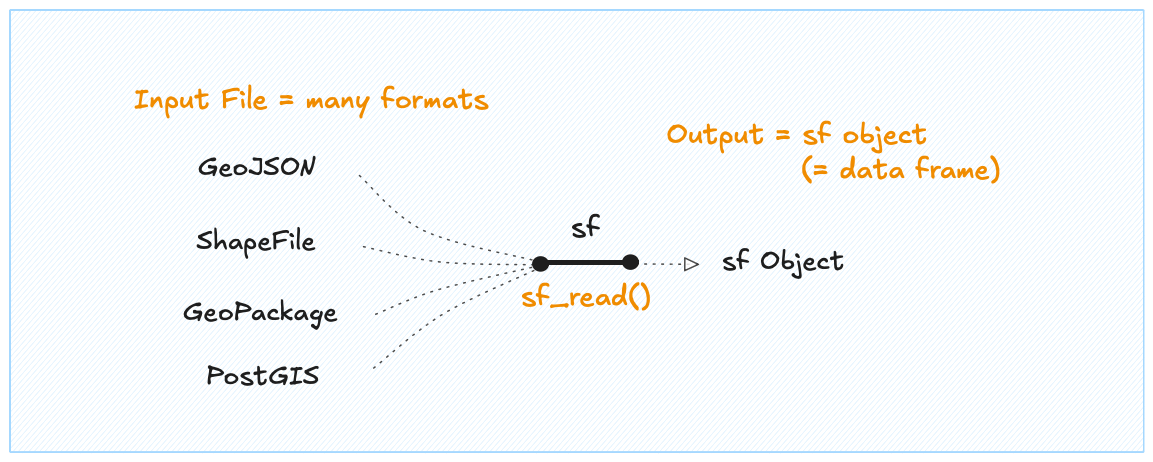
sf reads any spatial format and converts it into a standard R data frame, so you can work with it using the tools you already know.When you load a spatial dataset with st_read(), the returned sf object looks almost like a regular data.frame or tibble.
The only thing that makes an sf object different from a regular table is the additional "sticky" geometry column and metadata, following the universal approach outlined above:
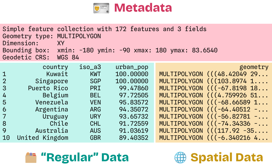
sf object is just a data frame with an extra sticky geometry column. Wrangle it as usual with base R or dplyr.No matter how much you subset, filter or transform your data, that column and the header stay attached so you never lose the link between your variables and their location on the map, and between the data entries and the metadata.
As it (mostly) behaves like a regular data frame, you can wrangle the data as usual, with base R commands like subset or dplyr verbs likefilter(), mutate(), andjoin(). You can also visualize it with ggplot2 using the same logic and syntax we already know 💙
Try it yourself: load and explore an sf object in R 👇
st_read().Notice the output above: even though we didn't explicitly select it, the geometry column is still there. This ensures that your spatial data remains "whole" as you clean and prepare your dataset for visualization.
🍊 The Peel Problem
To truly understand that CRS field in the metadata, we have to face an actual "translation problem": the Earth is a three-dimensional, slightly bumpy sphere, but our screens are flat.
Imagine drawing a map on an orange, then peeling it and trying to lay the skin perfectly flat on a table. You can't do it without tearing, stretching, or overlapping the pieces.
A Coordinate Reference System (CRS) is the mathematical recipe used to flatten that 3D surface into 2D coordinates. Because no recipe is perfect, every map involves a trade-off between shape, area, distance, and direction.
Geographic (GCS)
Treats the world as a sphere. Uses angular units (likely degrees) to define locations on a curved surface.
Spherical geometry is essential to calculate accurate measurements, as it accounts for the Earth’s actual shape rather than a flat map.
Projected (PCS)
The "flattened" version of our world. Converts degrees into linear units (such as meters or feet).
Projections are essential for 2D mapping. To avoid stretched or squashed visuals, we must choose a projection that fits our specific region.
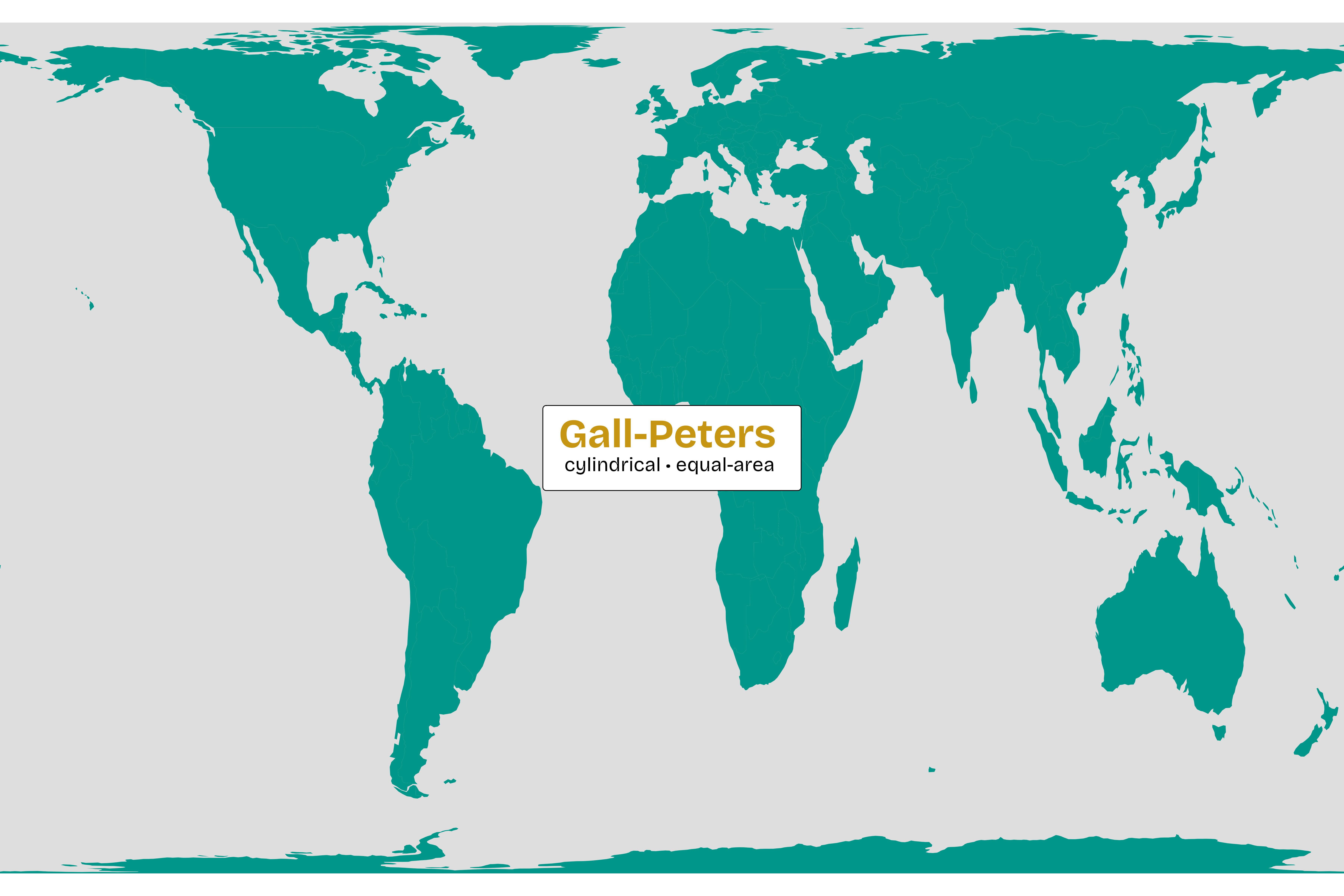
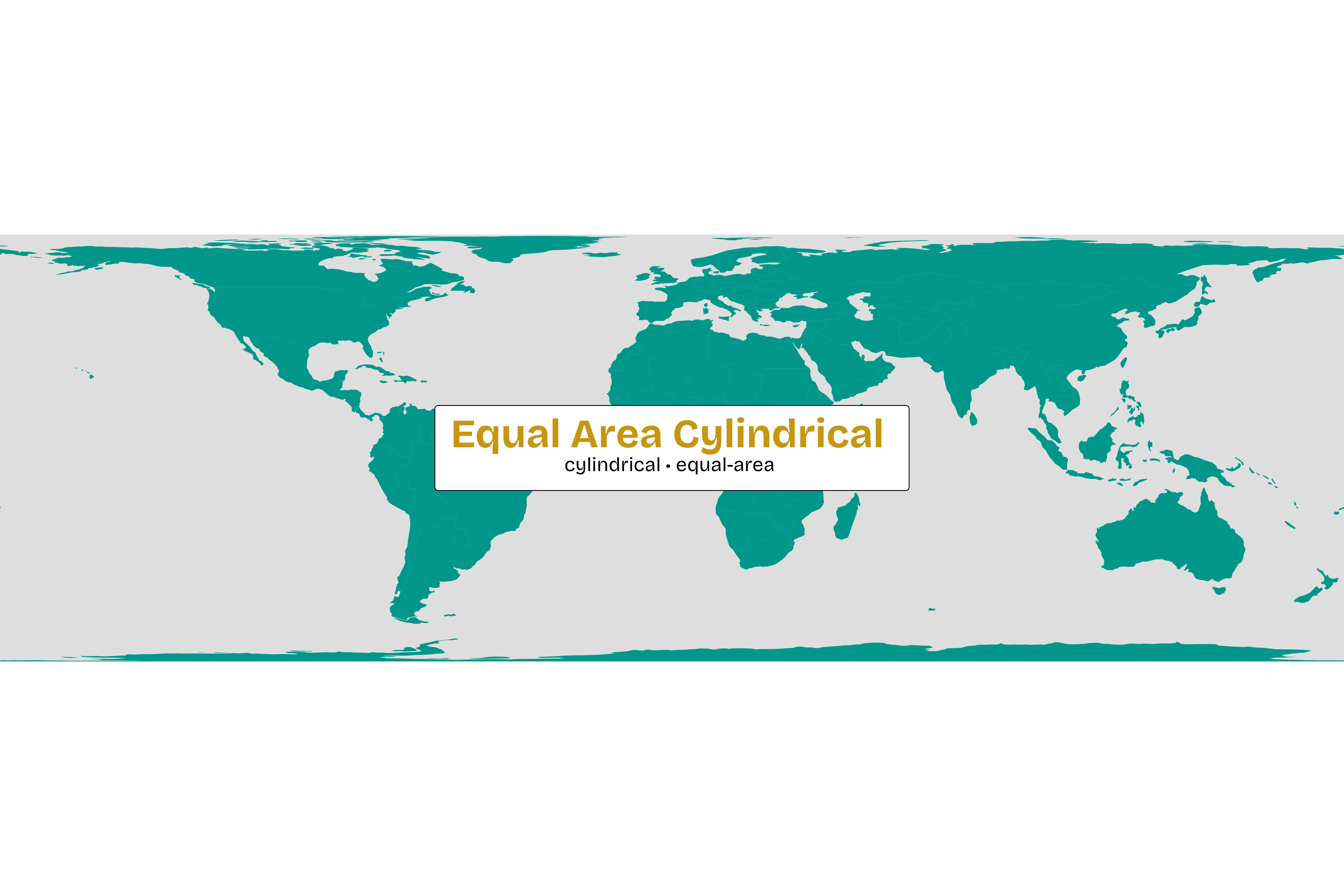
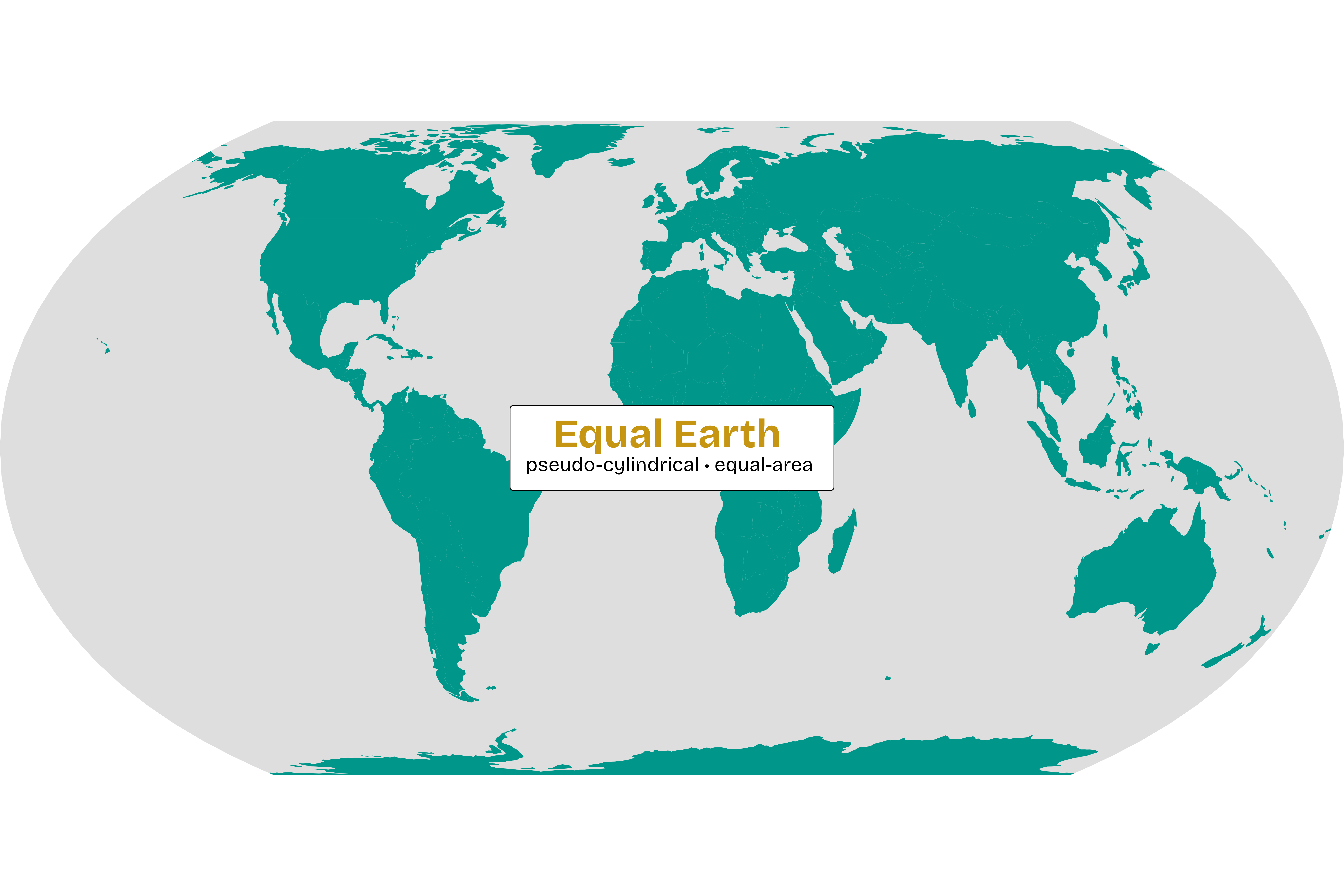
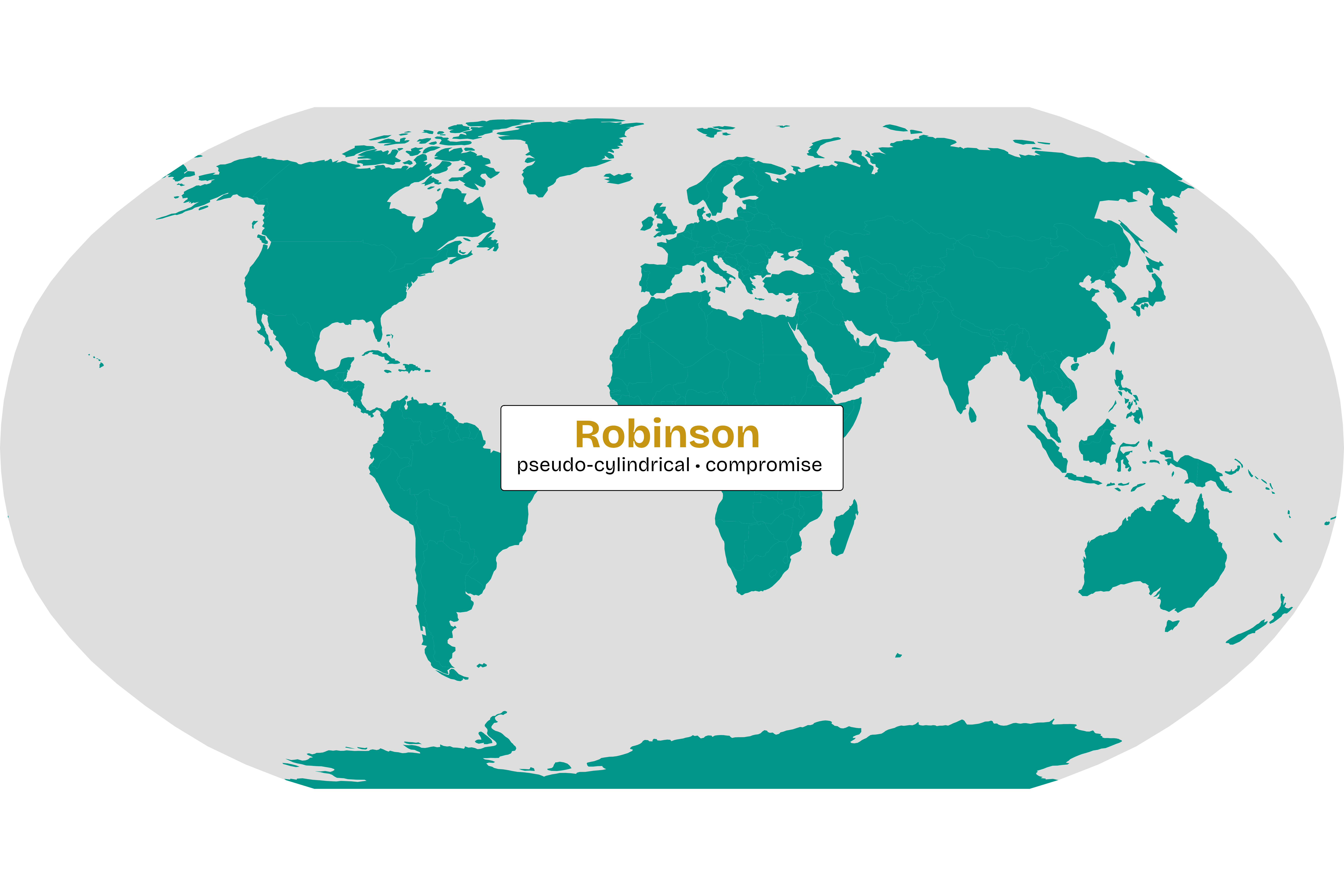
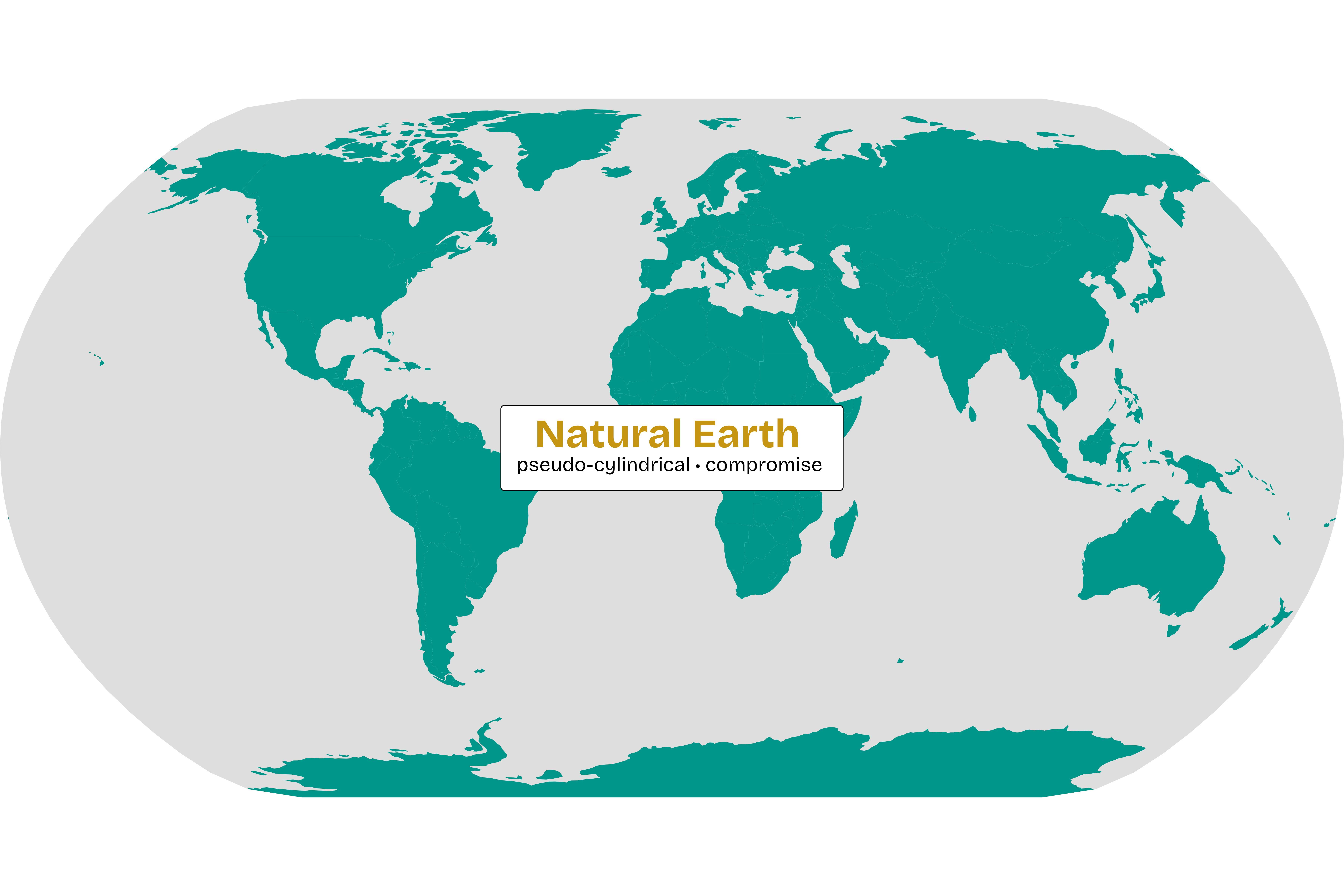
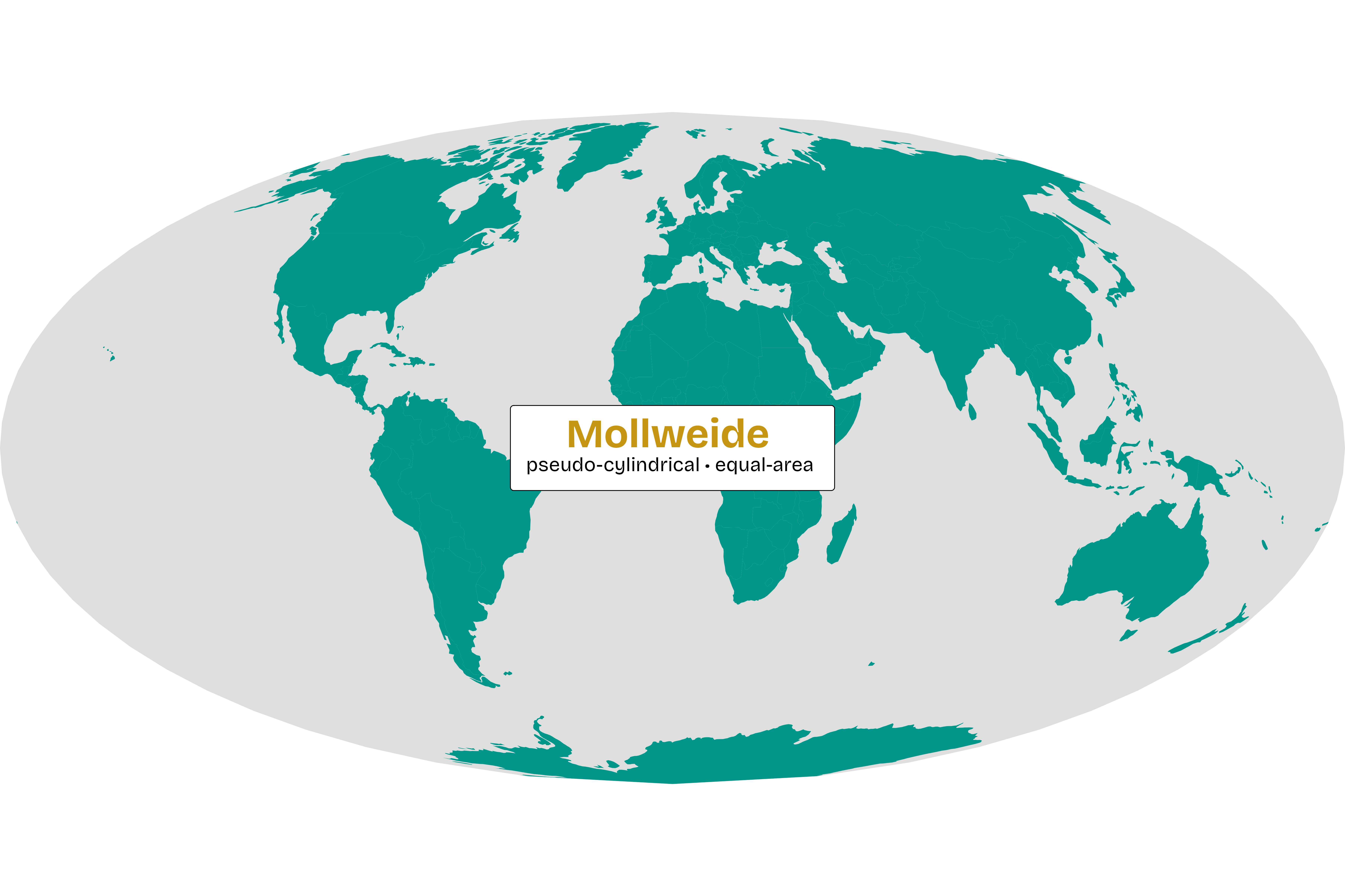
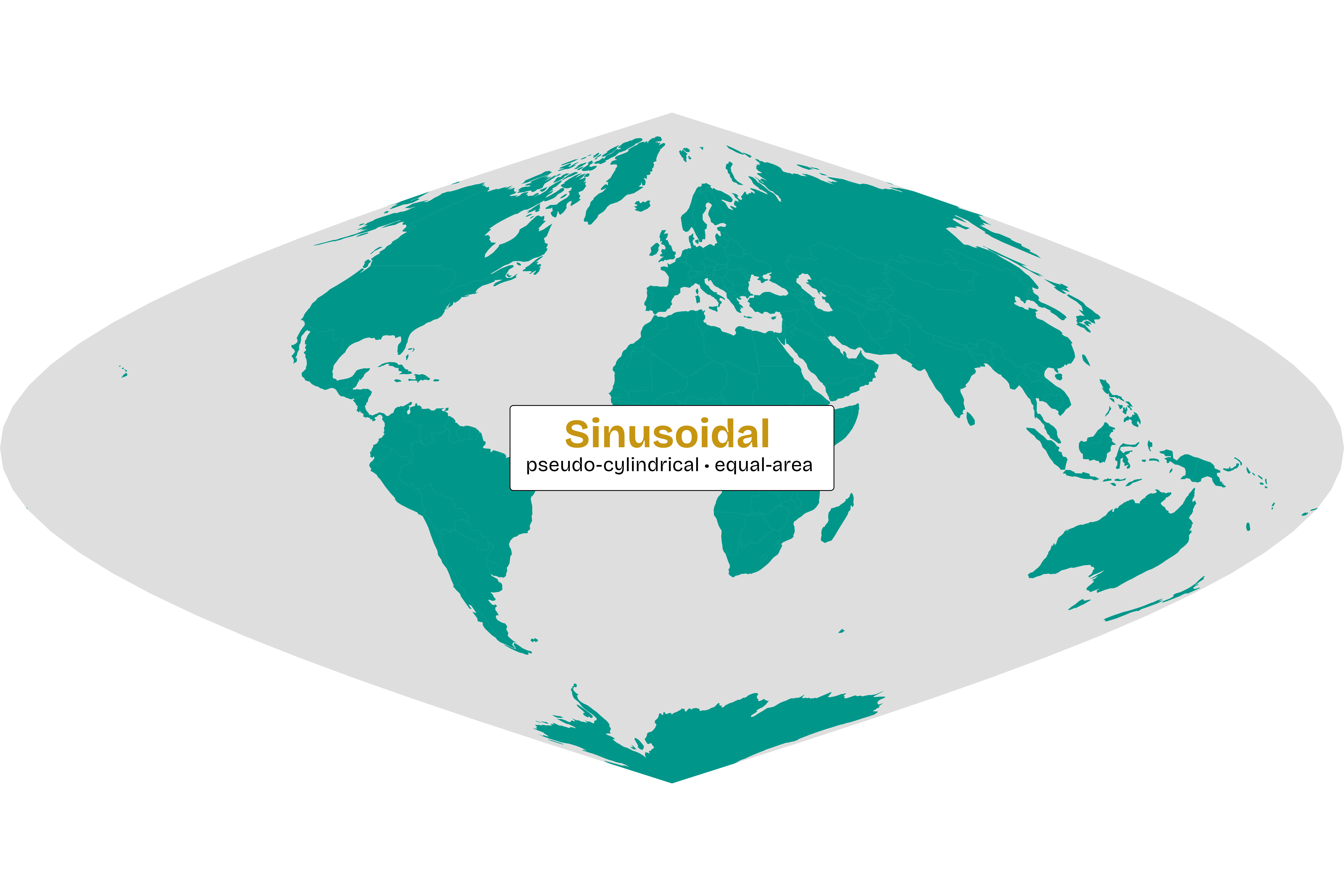
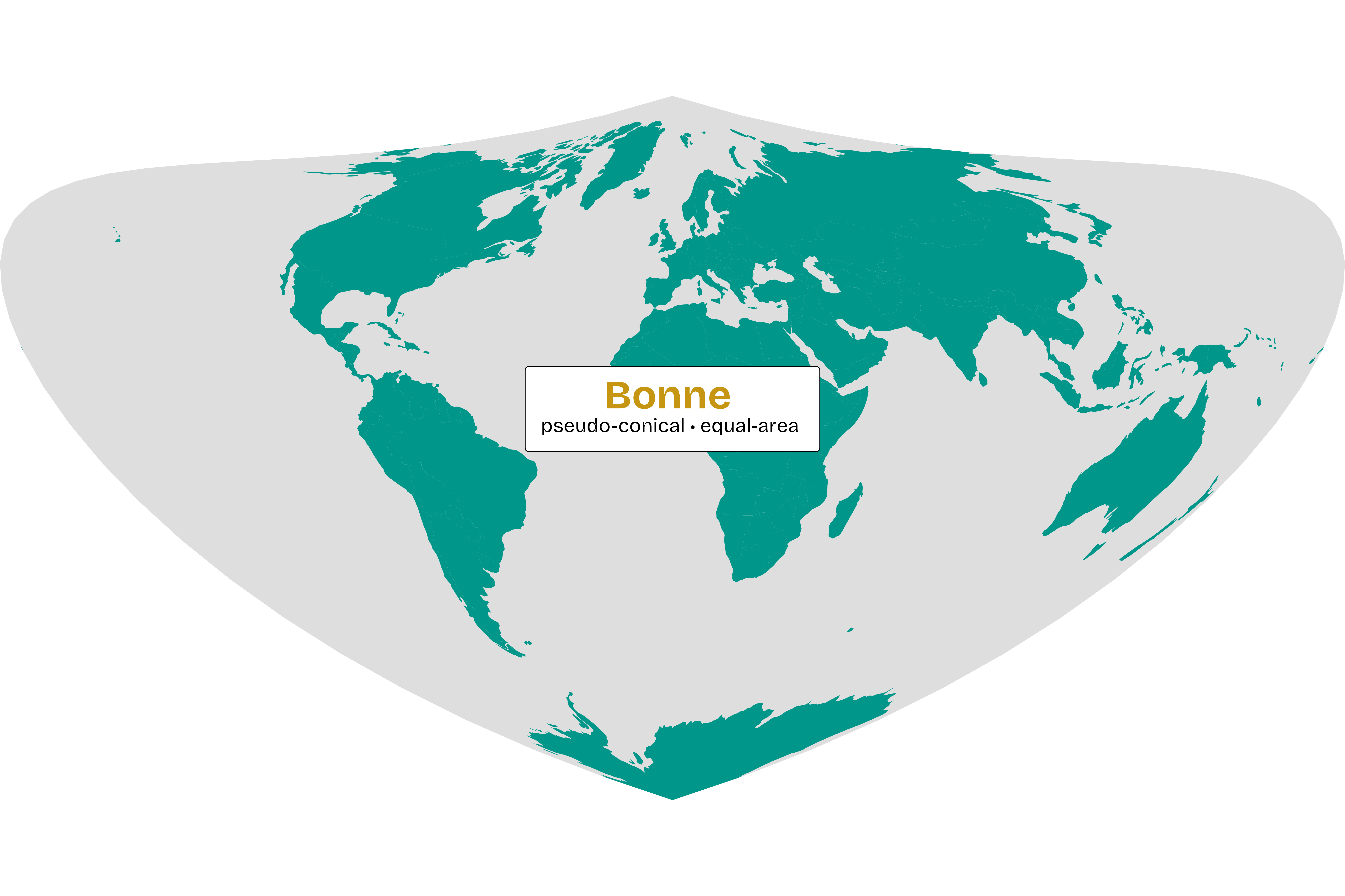
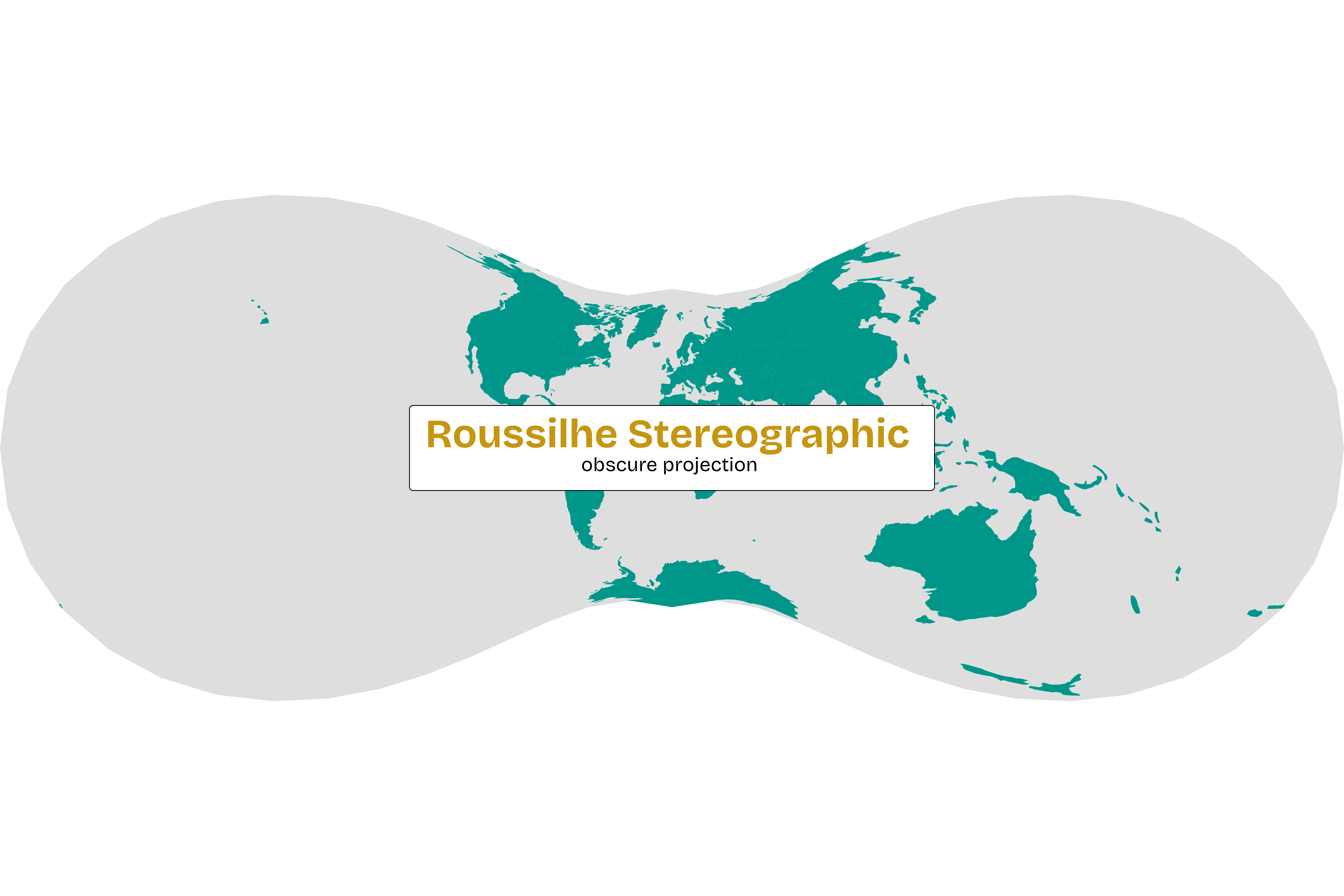
To showcase the "orange peel" problem, here are some popular, and a few less-common, projections that use different ways of flattening the world. Many wrap the globe around a cylinder to peel the skin, others use cones, planes or other obscure shapes to minimize distortions in specific regions.
Each projection prioritizes a specific measure: some are conformal (preserving shapes and angles), equal-area (preserving areas), or equidistant (preserving distances), while others use a compromise to balance these distortions.


The most famous "orange peel" compromise is the Mercator projection. It was designed for 16th-century sailors because it preserves straight lines for navigation, but it does so by stretching the poles.
On a Mercator map, Greenland looks as large as Africa.
But actually, Africa is 14 times larger than Greenland!
Looking at some of the equal-area projections in the carousel above, like Gall-Peters, Equal Earth, or Mollweide, the difference is immediate, though these come at the cost of distorting other measurements.
When visualizing data, using Mercator can unintentionally make northern countries look "more important" simply because they take up more pixels.
And because the mathematics behind these projections are incredibly dense, the mapping community uses shortcuts to project the world in a specific way.
🧮 The Math Behind the Map
The most common are EPSG codes : four or five-digit IDs that act like a lookup key for a specific projection recipe. For example, 4326 is the code for standard GPS coordinates (WGS84), while 3857 is the standard for web maps like those provided by Google or OpenStreetMap contributors.
While EPSG codes are the most common standard for identifying coordinate systems, you will occasionally see ESRI codes . Both serve the same purpose: they are simply different naming registries that often point to identical mathematical parameters.
In other use cases, you might encounter PROJ strings . These are long, cryptic lines of text starting with +proj=... that explicitly list every mathematical parameter of the projection (e.g., the datum, the units, and the central meridian) and offer granular control for custom map-making.
🎨 From Tables to Maps
The true power of the sf package isn't just how it stores data, but how easily it can be used in plotting libraries. Because the geometries are "sticky," R always knows exactly where each data point belongs on the canvas.
You've already mastered the grammar of graphics with ggplot2. And visualizing spatial data follows that exact same grammar. You don't need to learn a whole new language to make a map; you just need to learn one new layer and coordinate system that understand these geometric building blocks.
Now that you understand the 🪪 Spatial Passport and know about the 🧱 Building Blocks of spatial data, it's time to stop looking at rows of coordinates and start visualizing the world as we’ll put these concepts to work in the next lesson.
📚 Test Your Knowledge
To wrap up, check your understanding with a short quiz and see how well you’ve mastered the key ideas!
Which geometric structure is defined as a "series of points that close back on themselves as a ring"?
Why is the geometry column in an sf object referred to as "sticky"?
Following the "Simple Features" model, how should Japan be represented in a dataset of world countries?
To accurately represent area on a flat screen, what must happen to our 3D coordinates?
If you are sharing a Shapefile with a colleague, which of the following is true?
There exists a map that accurately represents shape, area, distance, and direction at the same time.