Exporting Plots: Saving High-Quality Graphics

🎞️ From Plot to Image

Sharing your plots effectively means more than just exporting an image. Correctly handling dimensions, resolution, and format ensures that your graphics remain sharp, readable, and visually consistent — whether they appear in papers, presentations, or online.

ggsave() does not only handle the name and format of the file (based on the extension, such as .png,.pdf, .svg), but lets you control the aspect ratio and resolution so the output looks crisp wherever it goes.

•  Format  — add a file extension to the name of your plot. Before choosing a specific file format, it helps to know the general distinction between raster and vector graphics:
  • Raster files (like png, jpg, and tif) are made of pixels, so enlarging them too much can make them blurry or blocky.

    ---

    Pick raster for web and on-screen use with appropriate pixel dimensions, e.g. 1200×800 px. Use higher resolution (~300–600 dpi) when preparing files for print sharing via social media or messengers.
    
    
  • Vector files (like pdf and svg) store shapes and lines, so they can be scaled infinitely without losing sharpness.

    ---

    Choose vector for print and post-editing in tools like Adobe Illustrator, Inkscape, or Figma. Avoid vector files when using very large datasets with millions of points (files can get heavy).
  
  
•  Aspect ratio  — control the aspect ratio by setting width and height (using values with "in" or "cm" as units). If you increase the plot size, geometries and theme elements will appear smaller.


•  Resolution (DPI)  — controls the pixel density of raster files. Does not apply to vector files, and is irrelevant for web graphics.

💾 Saving Plots

By default, ggsave() exports the last ggplot you generated, and places it in your current working directory. The extension decides the format — .png, .tif, .pdf, ... well, we covered that already.

You specify the file name and extension by passing it to the filename argument. If you want to store the plot in a different folder, you can specify:

• the full path pointing to the directory along with the name like "/Users/Emy/Project/plots/fig1.png", or starting with e.g. "C:/" on Windows (problematic when code is used on other machines!)
• a relative path like "plots/fig1.png" (relative to your current working directory). You can also add ./ for clarity, e.g. "./plots/fig1.png"
• a relative path built with file.path(), which safely combines directory and file names across operating systems, e.g. file.path("plots", "fig1.png")

Note: Windows uses the backslash \ in file paths, but in R this acts as an escape character. To avoid problems, use / or \\ instead — or simply use file.path() to build the path in a robust way.

You also can store a plot first and then hand over the ggplot object by specifying plot = as well.

Often, users rely on implicit matching here — the filename is provided first, so specifying the argument name (filename =) isn’t necessary, as shown in the second example above.

📐 Controlling the Export

When saving plots, it’s best to set the canvas explicitly so the file is ready for its final destination — whether that’s a paper, a slide deck, or the web.

First, control the  aspect ratio  by setting width andheight:

For raster formats like PNG or TIFF, you’ll also want to set the  resolution  with dpi (dots per inch):

Optionally, set the  background  explicitly with bg — helpful if your plot is placed over colored slide backgrounds or webpages:

🖨️ High-Quality Output

R uses a device to transform your R objects into images. But for professional publications, default devices may not always give the best results.

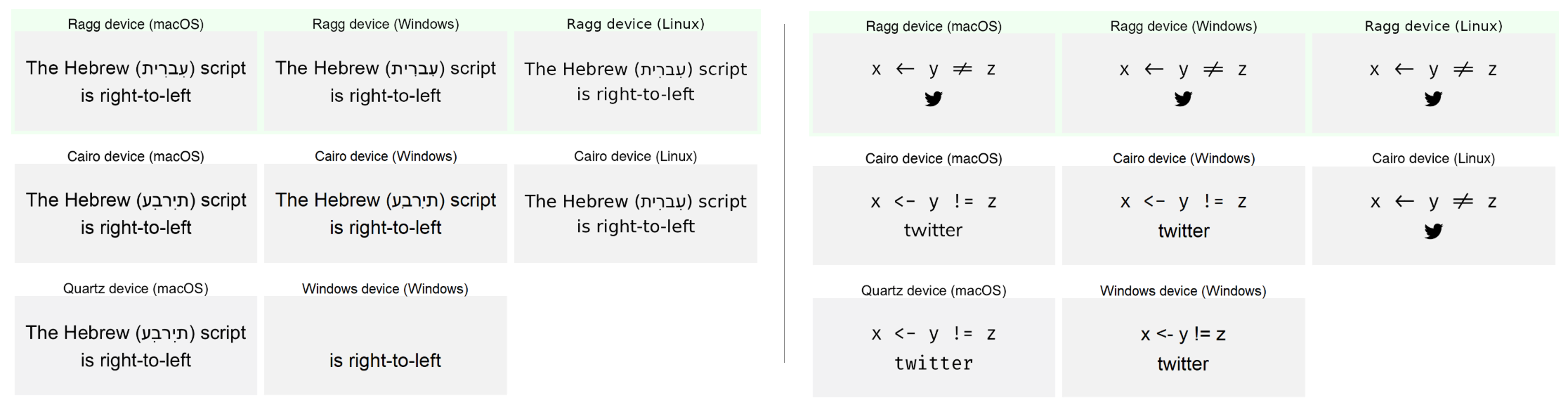
Issues can arise with custom typefaces, the depiction of symbols and emojis, and even subtle differences in rendering across formats or operating systems.

Two common solutions for high-quality output in R are AGG-based devices provided by the ragg 📦 and Cairo-based devices already included in base R’s grDevices (if R was built with Cairo support).

✨ Rendering Raster Files with ragg

The ragg package provides raster devices built on the AGG (Anti-Grain Geometry) rendering library, that is known for smooth anti-aliasing and reliable text output. It makes high DPI images easy to create and ensures fonts, symbols, emojis, and also right-to-left scripts render fast and consistently, even across platforms.

By default, ggsave() uses AGG-based devices now — if the ragg package is installed. To enable them, simply install the package with install.packages("ragg").

To specify it explictly, use the device argument:

✨ Rendering PDF Files with Cairo Devices

Cairo devices produce high-quality vector (and also raster) output with robust font and symbol support. It's ideal for plots with complex text, ligatures, or annotations, that are exported as PDF vector files.

You can render your PDF by specifying the cairo_pdf as device:

The graphics device backends has a huge impact on how your visualizations are rendered. The example below illustrates the differences, suming up nicely why choosing the right device matters for high-quality graphics — especially when running the code on different operating systems.

Live demo

This lesson was quite technical, and we believe it’s easier to follow when you see it in action. Here’s a video of Cédric saving a few charts and tackling some of the most common issues!

📋 Recap

We encourage you to open your own R environment and experiment with the concepts covered here. The usual in-course sandbox isn’t suited for this lesson.

To wrap up, check your understanding with a short quiz and see how well you’ve mastered the key ideas!